
Building a Reinforcement Learning Agent for Algorithmic Trading
- Thien @ AION Research
- Sep 29, 2024
- 11 min read
Updated: Sep 30, 2024
In this tutorial, we'll go through how to train a simple trading bot using reinforcement learning (RL) algorithms and neural network, with PyTorch and Stable Baselines 3 libraries. We'll focus mostly on the technical implementation, assuming some familiarity with RL theories and terminologies.
If you need to brush up on RL knowledge, these are 2 excellent resource:
Sutton, R. S., & Barto, A. G. (2018). Reinforcement learning: An introduction (2nd ed.). The MIT Press. for a comprehensive introduction to RL theory and mathematics.
OpenAI Spinning Up for a more hands-on walkthrough of deep learning based solutions
Disclaimer: The materials presented below for demo and educational purposes only and should not be used directly for real trading.
Framing the Reinforcement Learning Problem
Reinforcement learning centers around the process of teaching an AI agent to observe the environment and take appropriate actions, and in turn receiving rewards. In our case, the AI agent is a trading bot, the actions are buy, sell or hold, the observations are the prices time series and other trading data, and the rewards are profits from closed trades.

The above diagram is very popular in RL articles but it leads to a number of misconceptions. Neither the observations nor reward has to come externally from the environment but may consist of the agent's internal states and reward signals as well. In fact, rewards in RL algorithms, temporal difference (TD) learning in particular, correspond to the phasic response of dopamine neurons in neural science and cognitive psychology researches, which is completely internal. For our purpose here, it's ok to treat them as external like above but we can freely design the rewards in addition to trade profits to nudge the agent in certain directions.
RL problem and algorithms are often specified under the Markov Decision Process (MDP) framework, with a state St for the observations, a discrete or continuous variable At for the actions and a reward variable Rt. We'll use these terminologies onwards.
What "models" are needed for RL?
The objective for an RL agent is to take action given each state so as to maximize the sum of discounted future rewards. This sum of reward is referred to as value for each state or state-action pair. In our case, it is to maximize trading profits without going bankrupt first. To do this, we will train a policy function to map trade data to the best trade action (or exploratory action during learning) at every price bar.
RL technically doesn't require any model in the usual ML model sense. The term "model" in RL, as in model-based methods, refers to the world model that predicts state transitions probability and not the policy. The policy can even be a table that record values of state and actions (tabular methods) e.g. for simple problems with small set of states, actions and stationary reward distribution such as multi-armed bandit. Using a "model" for policy is referred to as function approximation method in RL. We can use any common supervised learning model for this, not just neural networks.
Actor-Critic Policy Architecture
For this project, we'll use a particular form of temporal difference learning called Actor-Critic. The critic component of the policy predicts the value of each state. The actor component optimizes for the value of each state-action pair by minimizing the TD-error from the immediate reward and the critic's predicted value of the next state. The system is designed this way to reduce variance in the recursive bootstrapping update in function approximation methods, which otherwise makes RL notoriously unstable and sample inefficient especially for off-policy training.

The main technical difference between RL and supervised learning (SL) appears in the bootstrapping policy function update using TD-error. Training errors for SL are from the difference between the model prediction and labels while TD-error also contains the model's own prediction as target. This makes RL much closer to the neural science of how humans and animals learn but also make it very problematic to train. The usual gradient descent back-propagation method for training SL model are not directly applicable. At the other end, the Monte Carlo types of RL methods which use full rollouts of an episodes to train is no difference from training SL models.
The state-action values are then converted into probability for each action to be taken, constituting a stochastic policy with built-in exploration. The on-policy variants of the actor-critic architecture are implemented in Stable Baselines 3 library through the advantage actor critic (A2C) and proximal policy optimization algorithms (PPO). They're both policy gradient methods where the critic is not exactly updated through state-action reward values described above but through the gradients of its policy function.
That's enough theory for now. Let's jump into the fun part!
Create a simulated environment
Let's first create a virtual environment and install the necessary libraries for this project. The the following command in your terminal from your project directory:
python -m venv ./venv
source ./venv/bin/activate
pip install stable_baselines3 statsmodels tensorboard
RL algorithms typically need a large amount of experience data in order to learn reliably well, so using only real prices data will not be enough. We'll generate time series data from pre-defined stochastic process instead. The following code wraps an ARMA time series data generation in a python iterable class:
Next we need to create a custom environment in the Gymnasium library that deliver observations and rewards to the agent at each time step. We call this BrokerEnv since it serves similar purposes to a trading broker. Define the following data structures to store data about our actions and states:
In BrokerState, we only keep a simple set of features. Equity is the trading account's total cash and asset value. There're 2 fields for currently open position size and its entry price, and the ts_buffer array stores the raw price data. In general, the agent would perform and learn better with additional engineered features in e.g. statistical features on the time series data etc. However, for a challenge and experimentation purpose, we'll only use raw price data, similar to how RL agent is trained to play games from raw gameplay images without any human curated features about the rules and strategies.
We can now create the custom gym's environment by deriving from the gym.Env class and fill out the following template:
In the init function, let's define a few variables and set the action space and observation space. Our broker environment uses a discrete action space with 3 values for hold, buy and sell, and a box space of float values for the observations as defined the state's class above.
In the reset function, we'd reset the price feed iterator and the state variable to its initial values:
Finally, we implement the step function that execute the broker's trading rules. This is assumed to happen at the end of each price bar:
Get the next closing price from the price feed.
Adjust the account's equity based on the price and terminate the episode with negative reward of the agent is bankrupted.
If the agent makes a buy or sell action with no open position, enter into a new position and deduct a transaction cost from the reward
If there's an open position, close the trade if the agent's action is not hold and then enter into a new one. Deduct transaction cost from the reward accordingly
For each closed trade, the reward is the difference between the current and entry price times the position size (negative size for short position)
Terminate the episode when the price feed is exhausted. No reward is given for any open trade.
Notice that we do not change the equity value when a position is entered or exited. This is because equity is the total sum of cash and asset values. Cash is converted into an asset with the same value when the position is entered and hence equity value remains the same. When the position is exited, equity is already adjusted by the latest price earlier on.
We store the raw price and reward into the info dictionary as well for logging and plotting purposes later on since the observation vector will be normalized for training. The full code for the custom environment class is as followed. We'll skip the render and close function for now.
Customize the policy neural network
With the broker environment defined above, we can already train an RL agent using stable baselines 3 built-in MLP's policy networks. This works pretty well when there're curated features available in the observation. However, we'll implement our own custom neural networks for the policy function to handle raw price data better. Stable Baseline's policy network is broken down into 2 stages: the feature extractor network and the actual policy network, both are customizable and can either be shared or separated for the actor and critic parts.

The default features extractor simply flattens the input observation vectors, which is more relevant for images data. We'll leave the feature extractor as is and only customize the policy network (in red). Define the following Pytorch's neural network module for our custom policy network as follow:
We applies 1D convolution layers on the raw price data. These will be shared between the actor and critic's networks. Afterwards, the embeddings from 1D conv layers are concatenated with the non time series features and passed to the MLP layers. Actor and critic have separate MLP layers. The number of layers, channels and units are parameterized to allow full customization when the model is instantiated. We use Tanh activation function mosly instead of the more common ReLU function since ReLU tends to results in more extreme outputs which is not suited for RL exploration and stochastic outputs.
Also note that we output only the latent representations from the actor and MLP. Stable baselines3 will add a last layer to convert to action probabilities and make sure the final outputs are appropriate for the given action space i.e. softmax for the actor's (pi) network and a linear layer for the value's (vf) network. Hence it's important to set our final MLP's output dimensions in the latent_dim_pi and latent_dim_vf instance variables so stable baselines could add the correct final layer.

Lastly, we create a class derived from stable baselines' ActorCriticPolicy class and set our custom policy network to the mlp_extractor variable to complete our customization:
Train and evaluate the RL agent
Training the policy network
Finally, we're now ready to train our trader RL agent. First, import necessary modules and prepare a few config and location to store the trained model artifacts:
For each trade, we'll long or short a fixed 100 units of the asset, costing about $100 per unit on average. Each trade direction costs 0.1% of the order's value in transaction fee, and so 0.2% total to enter and close a position. We use 30 bars look back for the time series observations.
To see whether the agent is able to learn the basic concept of buy low sell high, we prepare a synthetic covariance stationary ARMA time series like the above. The ideal trading strategy for this type of series is mean reversion. This type of series are not typical of direct financial instrument but are more representative of a series of spread for co-integrated assets in statistical arbitrage strategies.

Next, write the training function like so:
In the above code, we convert broker environment into a vector environment using the DummyVecEnv wrapper so that the system can learn multiple episodes in parallel. We also use the VecNormalize wrapper to normalize our observations data, similar to how we'd do features standardization in other ML models. Finally, we instantiate the Advantage Actor Critic (A2C) RL algorithm from Stable Baselines3, passing in the custom policy network class and train the agent for 500,000 times steps, with 1000 steps per episode.
The network architecture parameters are passed to the customized policy network class through the net_arch parameter. Here, we're building a very simple model with 2 small 1D convolution layers and 2 linear layers for the MLP.
We now run the above function to train the agent. The model artifacts are saved to the output/saved_model.zip file and the normalization parameters are saved to the output/vec_norm file.
model, env = train_model()Once the training is completed, we can start up Tensorboard to see how the learning curves look like. Run the following command in your terminal and follow the URL in the print out.
tensorboard --logdir ./tb_log
The training loss show gradual improvement over the training time steps but is still relatively unstable. We could probably improve more with further training but we'll move on for now. If your training curves looks a lot more noisy than the above, adjust the smoothing config in Tensorboard to make it easier to interpret.
Evaluate the RL Agent
Now, let's write a function to load our saved agent's policy model and see how much money it could make!
We run the agent for 100 episodes and calculate the profits earned per episode
Output:
...
#949 BUY -0.9768758821171336
#950 SELL 152.52442304544493
#951 BUY -0.9825159947823379
#952 SELL 18.50623998150767
#953 BUY -1.0161436929227023
#954 SELL -5.814759693974485
#955 BUY -0.9774159661785488
#956 SELL -43.003893575125076
#957 BUY -1.0012468637141425
2567.026599944372
The RL trader agent manages to make $2567 profit per episode, not too terrible!
We can modify the above code a bit to visualize trades on a price chart and understand its behaviour better.
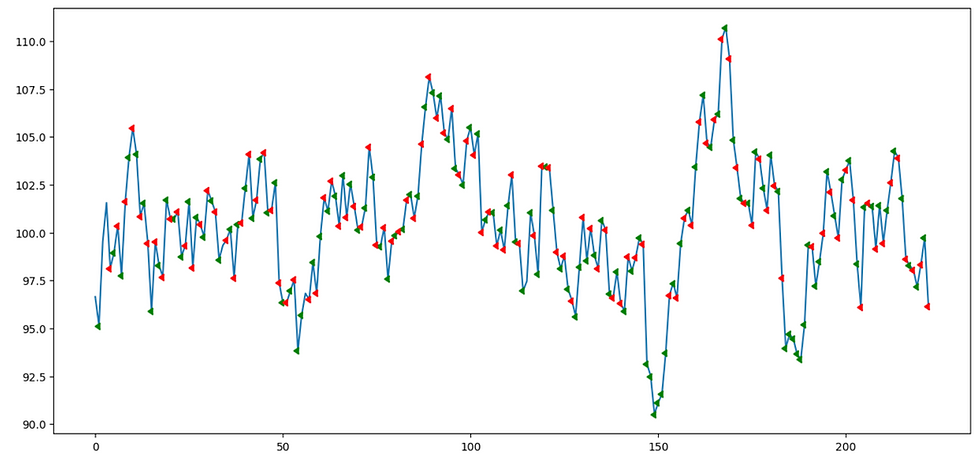
The agent seems to learn the basics of buy low sell high as most entries are followed by an exit when price moves in a favorable direction. There're also signs of a mean reversion strategy as most buy points are at negative deviations from the mean and sell points are at the positive deviation. However, the model seems to be over-trading, likely due to the well behaved nature of our idealized ARMA time series, relatively low transaction costs and abundant starting equity.
A more realistic example
Most financial assets don't behave like our idealized time series version above. In the equity sector of an efficient market, most stock price series behave more like a random walk stochastic process. A board stock market index or well-diversified portfolio, such as the S&P 500, is a random walk with positive drift to compensate for investor taking risks vs holding risk-free assets, according to theories such as capital asset pricing model. So far, they've behaved accordingly for the past 100 years, and hence the strategy for this is simply buy-and-hold or dollar cost averaging.
Let's see if our RL trader agent agrees or will it come up with something crazy! We first create a random walk versions for our price feed:
We increase the transaction cost to 0.02% per order and configure the time series generator to have parameters similar to the daily return drift and volatility of S&P 500, and change to 1 year of data per episode. Other parameters are kept similar to before
We then train the model using A2C algorithm similar to the step in the previous sections. Below are some logs from my own training and runs:
...
#55 BUY 170.63665365329183
#56 BUY -208.05512062108915
#57 BUY -178.02709379888788
#58 BUY 179.5132379902705
#59 BUY -143.7137424119343
#60 BUY 419.3480729541958
#61 BUY 325.7813776268587
#62 BUY 731.5016179027087
#63 BUY 939.0011712807978
#64 BUY -106.7044276461173
EP_RW_MEAN: 9904.464699896056
As expected, the agent mostly issue buy order due to the possible drift of the stochastic process. It also make to make $10,000 profit per year from it from 100 years simulation.
Let's see how well our RL agent do on real SPY data in the past 1 year. SPY is an index fund for the S&P 500, you can download daily price data from Yahoo Finance using the yfinance python library:
pip install yfinanceModify our load_model function to use the real SPY close price data as the price feed instead and run the RL agent trading.
Run the evaluation code similar to the steps in the previously section. My random walk trained RL agent manages to make about 9800 USD profit in the past 1 year. Not too shabby!
...
#210 BUY 443.28095703125
#211 BUY 268.6955200195313
#212 BUY 60.30060546875
#213 BUY 0.476979980468748
#214 BUY -188.8729296875
#215 BUY 932.2965576171875
#216 BUY -121.13087890625
#217 BUY 119.21149169921875
#218 BUY 140.14848876953124
#219 BUY -148.80257568359374
#220 BUY 203.10897705078125
#221 BUY -105.8605078125
#222 BUY 0
Total profits: 9810.313619995115
Conclusion
If you made it this far, congratulations! We've managed to build a working "profitable" algorithmic trading agent using state of the art reinforcement learning algorithms.
As we can tell from the above implementation of the RL trader agent that many real world trading conditions have been greatly simplified. We haven't incorporated more complicated market maker factors like slippage, bid-ask spread, liquidity etc. that will significantly impact profitability of a strategy. The agent employ a very simple neural networks and only have 3 actions to consider, using essentially only market order and not utilizing any other order types as risk management tools. There're still much room for improvements!
Most of the trading decisions that our RL agent does above can be similarly achieved using supervised learning or other statistical models. However, once many strategic decisions and complex optimization need to be integrated such as position sizing, risk management, derivative hedging, portfolio balancing, the RL framework could be handy.
Comentários